Calling Variants

The reads are now sorted, duplicates are flagged and the file is indexed. Calling variants means going along the genome and, at each position, deciding the sample's genotype from the reads that cover it. At most positions every read matches the reference. Where some don't, the caller has to decide whether the difference is real and, if it is, whether the sample carries it on one copy or both.

Reading the Pileup

Stacking up every read that covers a position gives a pileup, like the middle of Figure 5.1. At a heterozygous site, about half the reads should show the alternate allele. At a homozygous (alt) site, nearly all of them should.

Counting alone isn't enough, for three reasons:

• Sequencing errors. A few reads can differ from the reference just because the sequencer misread a base. The quality score of each base says how likely that is.
• Misplaced reads. A read with a low mapping quality might belong somewhere else, so its bases say little about this position. bcftools treats each base as no more reliable than its read's mapping quality (bcftools source).
• Chance. Which copy each fragment came from is random, like a coin toss. A heterozygous site covered by 30 reads shows exactly 15 of each allele only about one time in seven. Most of the time it shows somewhere between 10 and 20.

Genotype Likelihoods

Instead of counting, the caller asks a question for each possible genotype: if this were the sample's genotype, how likely would these exact reads be? The answer is the genotype likelihood (Li, 2011).

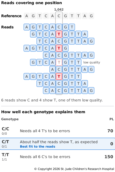
Figure 5.5 works through an example. At position 1,042 the reference has C, and ten reads cover it: six show C and four show T. One of the T's has a quality of Q10, and every other base is Q30.

• If the genotype were C/C, all four T's would have to be errors. Three errors at Q30 (1 in 1,000 each) and one at Q10 (1 in 10) together come to about 1 in 10 billion.
• If it were C/T, each read would be equally likely to show C or T, like a coin toss. The chance that all ten show exactly the bases they do is 1 in 1,024, about 1 in 1,000.
• If it were T/T, all six C's would have to be errors, about 1 in a billion billion.

C/T explains the reads about ten million times better than C/C. Callers write this comparison on the Phred scale as PL: the genotype that best fits the reads gets 0, and each other genotype gets 10 for every tenfold drop. Here PL is 70 for C/C, 0 for C/T and 150 for T/T. The low-quality T makes a difference: at Q30 it would raise C/C to 90. Real callers use a more detailed model, but the idea is the same.

Figure 5.5 Genotype likelihoods. Ten reads cover position 1,042, where the reference has C. For each possible genotype, the caller works out how likely these reads would be if that genotype were true. C/T fits them best, so its PL is 0. C/C would need all four T's to be errors, and T/T all six C's, so their PLs are higher: every 10 points means ten times less likely. The low-quality T could more easily be an error, so it costs C/C less. The data are made up.

PL describes only how well each genotype fits the reads, not how often variants turn up in the first place. Most positions in a genome match the reference, so the caller combines the likelihoods with a prior, a starting assumption that any one position probably matches the reference, to choose the genotype (bcftools documentation).

The caller also gives each call a QUAL score, which says how sure it is that the alternate allele is really there (VCF specification). QUAL is on the Phred scale, like base quality scores, so every 10 points means a tenfold smaller chance of being wrong. A QUAL of 10 means about a 1 in 10 chance that the variant isn't really there, 20 means 1 in 100 and 30 means 1 in 1,000. QUAL answers a different question from PL. PL compares the possible genotypes, while QUAL asks only whether the sample carries the alternate allele at all, on one copy or both. More reads showing the variant give stronger evidence, so QUAL tends to be higher where coverage is deeper. QUAL is also only as good as the caller's model. It can't account for problems the model doesn't know about, which is one reason the next page checks the calls against a truth set.

Indels

Indels go through the same steps, with one extra problem: the reads may not show them clearly. As described in Describing and Finding Indels, an aligner may write an indel near the end of a read as a few mismatches, or soft-clip it. bcftools works around this by collecting the indels that the reads suggest, building the local sequence with each one in place and realigning the nearby reads against each version to see which fits best (bcftools source). The genotype likelihoods then come from how well each read fits. Even so, indels are harder to call than SNVs, and the next page measures how much harder.

Other Ways to Call Variants

bcftools is a pileup caller: it looks at one position at a time. Two other approaches are widely used:

• Haplotype-based callers, such as GATK's HaplotypeCaller, look for regions that show signs of variation and reassemble the reads there into several candidate sequences for the region. They then work out how well each read fits each candidate, and which pair of candidates best explains the reads. The GATK team reports that this makes HaplotypeCaller more accurate where variants sit close together, and much better at indels than callers that look at one position at a time (GATK documentation).
• Deep learning callers, such as DeepVariant, turn the pileup around each possible variant into an image. A neural network trained on genomes whose variants are already known then decides the genotype. In its first paper, DeepVariant was more accurate than the existing tools it was compared with (Poplin et al., 2018).

We use bcftools here because it is small, quick and installs alongside samtools.

When a study sequences many samples, they are often called together, which is called joint calling. GATK, for example, first runs HaplotypeCaller on each sample separately, then genotypes them all together (GATK documentation). The result is one VCF that lists each variant found in the group, with every sample's genotype at that site.

Try It

This step needs chr20.fa from Setting Up and hg002.bam from Preparing Alignments. Run it from the same folder, with the reads-to-variants environment active:

# Build the pileup and genotype likelihoods, then call the variants
bcftools mpileup -f chr20.fa -r chr20:10000000-11000000 -a FORMAT/AD,FORMAT/DP -Ou hg002.bam \
  | bcftools call -m -v -Oz -o hg002.calls.vcf.gz
# Index the calls
bcftools index -t hg002.calls.vcf.gz

bcftools mpileup builds the pileup at each position and works out the genotype likelihoods. -r limits it to the region whose reads you downloaded, and -a FORMAT/AD,FORMAT/DP asks it to also record how many reads support each allele and how many it counted. -Ou passes its output through the pipe as BCF, the binary form of VCF, without compressing it, so the next tool can read it quickly. bcftools call -m chooses the genotypes, -v keeps only the sites with a variant and -Oz writes a compressed VCF.

bcftools prints a few notes as it starts. One says it assumes every site is diploid, with two copies, which is right for chromosome 20. Another says it reads at most 250 reads per position, far more than the 60 or so here. On our computer, the step took about four seconds.

Next, look at the calls themselves. bcftools view -H prints the calls without the file's header, and cut keeps seven of the columns:

# Show the first five calls, keeping seven of the columns
bcftools view -H hg002.calls.vcf.gz | head -n 5 | cut -f 1,2,4,5,6,9,10

Each line is one call. To show how to read a line, here is an example we made up:

chr20	10250320	C	T	222.4	GT:PL:DP:AD	0/1:255,0,255:47:25,22

From left to right, the columns are (VCF specification):

• chr20 and 10250320: the chromosome and the position.
• C and T: the reference allele and the alternate allele.
• 222.4: QUAL. This is far above 30, so the chance that this variant isn't really there is far smaller than 1 in 1,000.
• GT:PL:DP:AD: the names of the values in the last column, in order.

The last column, 0/1:255,0,255:47:25,22, holds the sample's values:

• 0/1: the genotype, heterozygous.
• 255,0,255: the PL for 0/0, 0/1 and 1/1. 255 is the largest value bcftools writes, so both other genotypes are at least that unlikely.
• 47: the depth, the number of reads counted here, not counting low-quality bases.
• 25,22: how many of those reads show each allele, 25 C and 22 T.

The columns skipped here, ID, FILTER and INFO, are described in VCF/BCF Files. Now read a few lines of your own output the same way. Then count the calls:

# Count the calls
bcftools view -H hg002.calls.vcf.gz | wc -l
# Count the SNVs
bcftools view -H -v snps hg002.calls.vcf.gz | wc -l
# Count the indels
bcftools view -H -v indels hg002.calls.vcf.gz | wc -l
# Count how many calls have each genotype
bcftools query -f '[%GT]\n' hg002.calls.vcf.gz | sort | uniq -c

There are 1,800 calls: 1,475 SNVs, which bcftools calls snps, and 325 indels. Of these, 1,111 are heterozygous (0/1) and 658 are homozygous for the alternate allele (1/1). The other 31 are 1/2, where each copy carries a different alternate allele, so the ALT column lists both.

Not all of these calls are right. The next page sets aside likely errors and checks the rest against HG002's truth set: Filtering and Checking Calls.