Introduction
Next Generation Sequencing ended with FASTQ files: millions of reads, each with a quality score for every base. On their own, those reads tell you very little. Nothing in a read says where in the genome it came from, and the few reads that differ from the reference are buried among millions that match it. FASTQ files are usually where the sequencing lab hands off and computational analysis picks up, and this chapter follows that analysis from reads to a list of variants.
Throughout, we use real reads from HG002, a person whose genome the Genome in a Bottle Consortium has studied in great detail, so you can check your results against a known answer.
Here, we focus on building a simple pipeline for germline single nucleotide variants and small insertions and deletions. A typical genome differs from the reference at about four to five million sites, and more than 99.9% of those variants are SNVs or short indels (1000 Genomes Project Consortium, 2015). Other kinds of variants, such as somatic, structural and copy number variants, would each need a chapter of their own, which we don't have space for here.
Getting from reads to variants takes four steps:
- Map each read to the place in the reference genome it most likely came from.
- Prepare the alignments: sort them by position, flag reads that are copies of the same original fragment, and build an index so tools can jump straight to any region.
- Call variants: at each position, weigh the evidence in the reads and decide the genotype.
- Filter and check: set aside calls that are probably wrong, then measure how accurate the rest are by comparing them with a truth set, a list of variants already known for the same sample.
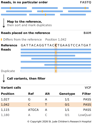
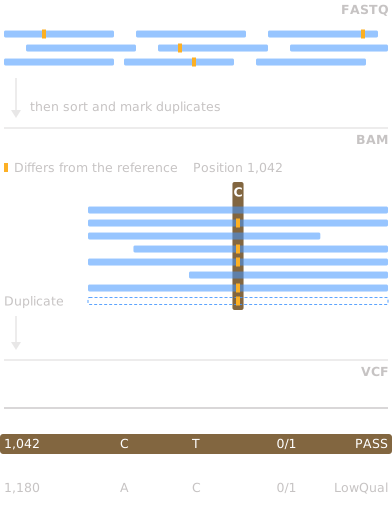
Along the way the data moves through three file formats: FASTQ for reads, BAM for reads placed on the reference, and VCF for variant calls. These pages explain just enough of each to follow along, and Genomic File Formats covers them in full.
Try It Yourself
Each step ends with a Try It section that runs it on HG002's reads. Because the exercise uses a small piece of one chromosome, it needs only a terminal on macOS or Linux (on Windows, use the Windows Subsystem for Linux), about 500 MB of disk space and a few minutes.
In This Chapter
- Setting Up: installing the tools and downloading the data for the Try It sections.
- Read Mapping: finding where in the genome each read came from.
- Preparing Alignments: sorting, marking duplicates and indexing.
- Calling Variants: deciding the genotype at each position from the reads that cover it.
- Filtering and Checking Calls: setting aside likely errors, and measuring how well the calls match a truth set.
- Conclusion: what the pipeline did, and how real analyses go further.